Comparing Join Implementations

In the upcoming SIGMOD the group around Jens Dittrich as a very nice paper about different join implementations: Stefan Schuh, Xiao Chen, Jens Dittrich. An Experimental Comparison of Thirteen Relational Equi-Joins in Main Memory. SIGMOD 2016.
And, as the title implies, it brings light into the overwhelming landscape of papers about join implementations.  It does a pretty good job of pointing out classical implementation choices, and then compares them using not only micro-benchmarks but also using TPC-H Query 19.

And this is a very important contribution. Many papers only consider micro-benchmarks for join experiments, but this is often not very helpful to derive the overall impact of a join implementation for complex queries. This paper does much better.

Still, I am not 100% satisfied with the comparison, which brings me to this blog post here. There are two aspects that I would like to emphasize: First, what is actually a typical join problem? And second, how should we interpret the performance of different join implementations?
Note that even though I will argue against some of the conclusions from the SIGMOD paper, this is not meant as a critique of the paper itself. Stefan Schuh at al. do a good job there, I just disagree a bit with how we should interpret the results.


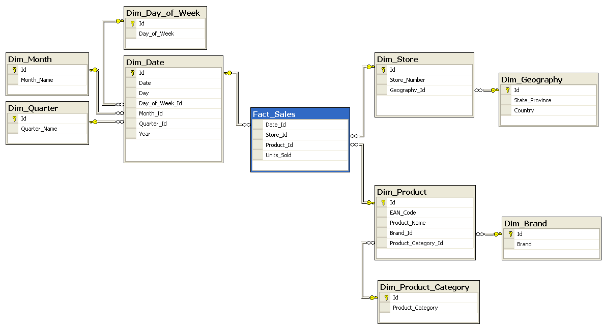
Coming to my first point, what is a typical join problem? Most papers that consider partitioning join implementations, including the current one, consider joins between relations of similar sizes. In Figure 9 and 10 the authors show results for R⨝S where |S|=|R| and where |S|=10*|R|. Which seems to span a wide range of cardinalities. But is this realistic? If we consider a typical star or snowflake schema like this one

we notice that 1) the cardinality differences between connected relations can be very large, and 2) they will be even larger once query predicates are introduced. Many data warehouse queries will filter one or more dimensions and then join that with the huge facts table.

Of course not every database has a star or snowflake schema. In particular, TPC-H does not. But even there, when looking across all 22 TPC-H queries, 97.4% of the joined tuples occur on the probe side. In fact I would argue that, due to filter predicates, most joins will be between relations of very different sizes. Which makes partitioning joins a lot less attractive, but which is often ignored by papers about that kind of joins.
Of course it might make sense to have different join implementations available, to handle the |S|=|R| case more efficiently. But one should keep in mind that this case is an exception rather than the norm.



Another question I would like to emphasize is, how should we interpret the performance of different join implementations? Query performance is a complex beast with many different metrics like cache-miss stalls, instructions per cycle, branch misses etc. I would argue that if you compare different approaches, the only sane metric is the overall execution time. It is the only sane one because 1) we are waiting for the query result after all, and 2) the individual metrics are often misleading for the overall performance. In fact that there can be approaches that are worse than the competitors in all the previously mentions metrics, but are faster overall.

In the paper the authors show performance results for TPC-H Q19, which consists of a single join between lineitem and part, followed by simple summation without group by attributes. If we look at Figure 14

We see that, overall, NOP, i.e., a non-partitioning join, is the fastest for this query. Still, the authors argue that NOP is the slowest of all four alternatives, because the colored bar of it is the highest. I tend to believe that this is an artifact of measurement of the colored bars: They were computed by running the joins on pre-filtered input, without the subsequent aggregation. But that experimental setup ignores a major weakness of the partitioning joins, namely that they often lead to massively random access after the join.
All joins were implemented as tid-joins, i.e., not the tuples themselves were passed around but only references to the original tuple. This is important for the partitioning joins, as otherwise the partitioning phase becomes very expensive. But as a consequence, the missing attributes have to be looked up afterwards. For the NOP join the accesses to lineitem are sequential, while for the partitioning joins these accesses are in more or less random order, which is quite expensive. Therefore the colored bars, which lack the attribute accesses, are misleading.

Which brings me back to my original point, namely that the only really sane metric is the overall execution time. Of course it would be nice to know which fraction of the query execution time would be spend in the join, or how some individual metrics are affected by a certain join implementation. But in reality we cannot answer these questions because there is a very complex interaction between implementations and the rest of the execution pipeline. The only thing we can measure reasonably well is the overall time.


Note that I do not want to criticize the paper for the before mentioned points. It does a very fine job of comparing different approaches, and I strongly recommend you to read it. I would have wished for a slightly different emphasis in the conclusion, but that is of course just my own opinion. I am looking forward for hearing the talk at SIGMOD!