Making unwinding through JIT-ed code scalable

 Exceptions are a very handy mechanism to propagate errors in C++ programs, but unfortunately they do not scale very well. In all common C++ implementations the unwinding mechanism takes global lock during unwinding, which has disastrous consequences when the number of threads is high. On a machine with 256 hardware context we see worse-than-single-threaded behavior even for relatively modest failure rates.

Fortunately the Florian Weimer fixed one contention point in gcc 12 on systems with glibc 2.35 or newer, which gives us scalable exceptions as long as no JIT-ed code has been registered. Unfortunately our system does register JIT-ed code... Which means exception unwinding in our code base is still single-threaded in practice.

But we can fix that by teaching gcc to store the unwinding information in a read-optimized b-tree, which allows for fully parallel unwinding without any atomic writes. There is a gcc patch that does just that, but unfortunately it is quite involved and difficult to review. This article series thus explains all parts of the patch and shows how a read-optimized b-tree can be implemented lock-free. 

In order to keep the article length somewhat reasonable, the discusses is broken into parts:

1. The problem (this article)
2. Replacing the gcc hooks 
3. Optimistic Lock Coupling
4. The b-tree 
5. b-tree operations  
   

When unwinding exceptions, the compiler has to find the corresponding unwinding information for every call frame on the stack between the throw and the catch. gcc uses two different mechanisms for that: For ahead-of-time compiled code it asks glibc to find the unwinding information using either dl_iterate_phdr (on older systems) or _dl_find_object (on systems with glibc 2.35 or newer). Note that this mapping is not static, as shared libraries could be added or removed at any time, potentially during a concurrent unwind. For that reason dl_iterate_phdr was protected by a global mutex, which clearly does not scale. _dl_find_object avoids that mutex by using a lock-free data structure. But that only affects ahead-of-time compiled code, for JITed code libgcc uses a different mechanism, which we now discuss:

For JITed code the emitter has to explicitly register the unwinding information using __register_frame_info_bases (and the very similar __register_frame_info_table_bases):

void
__register_frame_info_bases (const void *begin, struct object *ob,
			     void *tbase, void *dbase)
{
  /* If .eh_frame is empty, don't register at all.  */
  if ((const uword *) begin == 0 || *(const uword *) begin == 0)
    return;

  ob->pc_begin = (void *)-1;
  ob->tbase = tbase;
  ob->dbase = dbase;
  ob->u.single = begin;
  ob->s.i = 0;
  ob->s.b.encoding = DW_EH_PE_omit;
#ifdef DWARF2_OBJECT_END_PTR_EXTENSION
  ob->fde_end = NULL;
#endif

  init_object_mutex_once ();
  __gthread_mutex_lock (&object_mutex);

  ob->next = unseen_objects;
  unseen_objects = ob;
#ifdef ATOMIC_FDE_FAST_PATH
  /* Set flag that at least one library has registered FDEs.
     Use relaxed MO here, it is up to the app to ensure that the library
     loading/initialization happens-before using that library in other
     threads (in particular unwinding with that library's functions
     appearing in the backtraces).  Calling that library's functions
     without waiting for the library to initialize would be racy.  */
  if (!any_objects_registered)
    __atomic_store_n (&any_objects_registered, 1, __ATOMIC_RELAXED);
#endif

  __gthread_mutex_unlock (&object_mutex);
}

 Which conceptually is a simple thing: It grabs a mutex, puts the object information into a list, and released the mutex. Note the code within the ATOMIC_FDE_FAST_PATH block: As we will see below, that unwinding mechanism is very slow. Thus, libgcc tries to avoid taking that path by remembering if any JITed code was registered at all. If not, it stops unwinding immediately. But that mechanism does not help if we do have JITed code.

During unwinding, the unwinder calls  _Unwind_Find_FDE, which traverses the list in order to find the corresponding unwind table for the given address:

const fde *
_Unwind_Find_FDE (void *pc, struct dwarf_eh_bases *bases)
{
  struct object *ob;
  const fde *f = NULL;

#ifdef ATOMIC_FDE_FAST_PATH
  /* For targets where unwind info is usually not registered through these
     APIs anymore, avoid taking a global lock.
     Use relaxed MO here, it is up to the app to ensure that the library
     loading/initialization happens-before using that library in other
     threads (in particular unwinding with that library's functions
     appearing in the backtraces).  Calling that library's functions
     without waiting for the library to initialize would be racy.  */
  if (__builtin_expect (!__atomic_load_n (&any_objects_registered,
					  __ATOMIC_RELAXED), 1))
    return NULL;
#endif

  init_object_mutex_once ();
  __gthread_mutex_lock (&object_mutex);

  /* Linear search through the classified objects, to find the one
     containing the pc.  Note that pc_begin is sorted descending, and
     we expect objects to be non-overlapping.  */
  for (ob = seen_objects; ob; ob = ob->next)
    if (pc >= ob->pc_begin)
      {
	f = search_object (ob, pc);
	if (f)
	  goto fini;
	break;
      }

  /* Classify and search the objects we've not yet processed.  */
  while ((ob = unseen_objects))
    {
      struct object **p;

      unseen_objects = ob->next;
      f = search_object (ob, pc);

      /* Insert the object into the classified list.  */
      for (p = &seen_objects; *p ; p = &(*p)->next)
	if ((*p)->pc_begin < ob->pc_begin)
	  break;
      ob->next = *p;
      *p = ob;

      if (f)
	goto fini;
    }

 fini:
  __gthread_mutex_unlock (&object_mutex);

  if (f)
    {
      int encoding;
      _Unwind_Ptr func;

      bases->tbase = ob->tbase;
      bases->dbase = ob->dbase;

      encoding = ob->s.b.encoding;
      if (ob->s.b.mixed_encoding)
	encoding = get_fde_encoding (f);
      read_encoded_value_with_base (encoding, base_from_object (encoding, ob),
				    f->pc_begin, &func);
      bases->func = (void *) func;
    }

  return f;
}

In the fast path it tries to stop early if no unwinding information had been registered. But if any unwinding frame has been registered by JITed code, it grabs the global object_mutex and does everything effectively single-threaded. This does not scale. Thus, we discuss how to switch gcc to a lock-free lookup structure in the next article.

Cloud Network Traffic Within the Same Region Can Be Very Expensive

Everyone knows that the major cloud vendors try to make it easy to get data in, and hard to get it out. What is less known is that high egress cost also applies to outbound traffic within the same region.

Let's look at AWS specifically. In AWS, EC2 outbound traffic is only free within the same availability zone (AZ). Moving data from one AZ to another in the same region is actually quite expensive:

"IPv4: Data transferred “in“ to and “out“ from Amazon EC2 [...] across Availability Zones in the same AWS Region is charged at $0.01/GB in each direction." source

This means that transferring 1TB costs $0.01/GB * 1000GB * 2 = $20. For comparison: most inter-region transfers cost $0.02 per GB, but only for outgoing traffic. Thus, remarkably, transferring 1TB from Ohio to Tokyo will cost the same as transferring it within Ohio from us-east-2a to us-east-2b. Two c5n.18xlarge instances communicating with each other at full 100 Gbit speed can theoretically incur network costs of $1,800 per hour (or $1,296,000 per month).

Interestingly, S3 can be used to bypass the high traffic cost when moving data between different AZs in the same region because

"Data transferred directly between Amazon S3 [...] in the same AWS Region is free." source

Let's see if we can exploit this. Consider again our example where we want to transfer 1TB from us-east-2a to us-east-2b. Instead of two EC2 instances talking directly, we could use an S3 Standard bucket in us-east-2. We first PUT the data into it from us-east-2a, then GET the data from that bucket using us-east-2b instances, and finally delete all objects. If we split our data into 1,000 1GB chunks, we need to pay for only 1,000 PUT and 1,000 GET S3 requests, which would be less than $0.01. Storage cost is also low: assuming a transfer rate of 1GB/s, the data would have to be stored in S3 for less than an hour, which costs about $0.03 (and could be reduced via pipelining). Thus, in total we can transfer 1TB through S3 for less than $0.05 instead of $20.

To summarize, inter-AZ traffic cost within the same region is unreasonably expensive. It seems unlikely that these prices have any resemblance to internal AWS cost -- as is reflected by the fact that AWS services such as S3 allow bypassing this cost.

Are you sure you want to use MMAP in your database management system?

Many database management systems carefully manage disk I/O operations and explicitly cache pages in main memory. Operating systems implement a page cache to speed up recurring disk accesses as well, and even allow transparent access to disk files through the mmap system call. Why do most database systems then even implement I/O handling and a caching component if the OS provides these features through mmap? Andrew Pavlo, Andrew Crotty, and myself tried to answer this question in a CIDR 2022 paper. This is quite a contentious question as the Hacker News discussion of the paper shows.

The paper argues that using mmap in database systems is almost always a bad idea. To implement transactions and crash recovery with mmap, the DBMS has to write any change out-of-place because there is no way to prevent write back of a particular page. This makes it impossible to implement classical ARIES-style transactions. Furthermore, data access through mmap can take a handful of nanoseconds (if the data is in the CPU cache) or milliseconds (if it's on disk). If a page is not cached, it will be read through a synchronous page fault and there is no interface for asynchronous I/O. I/O errors, on the other hand, are communicated through signals rather than a local error code. These problems are caused by mmap's interface, which is too high-level and does not give the database system enough control.

In addition to discussing these interface problems, the paper also shows that Linux' page cache and mmap implementation cannot achieve the bandwidth of modern storage devices. One PCIe 4.0 NVMe SSD can read over 6 GB/s and upcoming PCIe 5.0 SSDs will almost double this number. To achieve this performance, one needs to schedule hundreds or even thousands (if one has multiple SSDs) of concurrent I/O requests. Doing this in a synchronous fashion by starting hundreds of threads will not work well. Other kernel-level performance issues are single-threaded page eviction and TLB shootdowns. Overall, this is an example of OS evolution lagging behind hardware evolution.

The OS has one big advantage over the DBMS though: it has control over the page table. Once a page is mapped, accessing it becomes transparent and as fast as ordinary memory. Any manually-implemented buffer manager, in contrast, will have some form of indirection, which causes some overhead. Pointer swizzling as implemented in LeanStore and Umbra is a fast alternative but is also more difficult to implement than a traditional buffer manager and only supports tree-like data structures. Therefore, an interesting question is whether it would be possible to have an mmap-like interface, but with more control and better performance. Generally I believe this kind of research between different areas should be more common.

 

AWS EC2 Hardware Trends: 2015-2021

 

Over the past decade, AWS EC2 has introduced many new instance types with different hardware configurations and prices. This hardware zoo can make it hard to keep track of what is available. In this post we will look at how the EC2 hardware landscape changed since 2015. This will hopefully help picking the best option for a given task.

In the cloud, one can trade money for hardware resources. It therefore makes sense to take an economical perspective and normalize the hardware resource by the instance price. For example, instead of looking at absolute network bandwidth, we will use network bandwidth per dollar. Such metrics also allow us to ignore virtualized slices, reducing the number of instances relevant for the analysis from hundreds to dozens. For example, c5n.9xlarge is a virtualized slice of c5n.18xlarge with half the network bandwidth and half the cost.

Data Set

We use historical data from https://instances.vantage.sh/ and only consider current-generation Intel machines without GPUs. All prices are for us-east-1 Linux instances. Using these constraints, in July 2021 we can pick from the following instances:

name	vCPU	memory [GB]	network [Gbit/s]	storage	price [$/h]
m4.16x	64	256	25		3.20
h1.16x	64	256	25	8x2TB disk	3.74
c5n.18x	72	192	100		3.89
d3.8x	32	256	25	24x2TB disk	4.00
c5.24x	96	192	25		4.08
r4.16x	64	488	25		4.26
m5.24x	96	384	25		4.61
c5d.24x	96	192	25	4x0.9TB NVMe	4.61
i3.16x	64	488	25	8x1.9TB NVMe	5.00
m5d.24x	96	384	25	4x0.9TB NVMe	5.42
d2.8x	36	244	10	24x2TB disk	5.52
m5n.24x	96	384	100		5.71
r5.24x	96	768	25		6.05
d3en.12x	48	192	75	24x14TB disk	6.31
m5dn.24x	96	384	100	4x0.9TB NVMe	6.52
r5d.24x	96	768	25	4x0.9TB NVMe	6.91
r5n.24x	96	768	100		7.15
r5b.24x	96	768	25		7.15
r5dn.24x	96	768	100	4x0.9TB NVMe	8.02
i3en.24x	96	768	100	8x7.5TB NVMe	10.85
x1e.32x	128	3904	25	2x1.9TB SATA	26.69

Compute

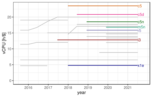
Using our six-year data set, let's first look at the cost of compute:

It is quite remarkable that from 2015 to 2021, the cost of compute barely changed. During that six-year time frame, the number of server CPU cores has been growing significantly, which may imply that Intel compute power is currently overpriced in EC2. In the last couple of years EC2 has introduced cheaper AMD and ARM instances, but it's still surprising that AWS chose to keep Intel CPU prices fixed.

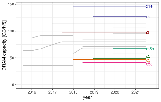
DRAM Capacity

For DRAM, the picture is also quite stagnant:



The introduction of the x1e instances improved the situation a bit, but there's been a stagnation since 2018. However, this is less surprising than the CPU situation because DRAM commodity prices in general did not move much.

Instance Storage

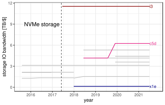
Let's next look at instance storage. EC2 offers instances with disks (about 0.2GB/s bandwidth), SATA SSDs (about 0.5GB/s bandwidth), and NVMe SSDs (about 2GB/s bandwidth). The introduction of instances with up to 8 NVMe SSDs in 2017 clearly disrupted IO bandwidth speed (the y-axis unit may look weird for bandwidth but is correct once we normalize by hourly cost):



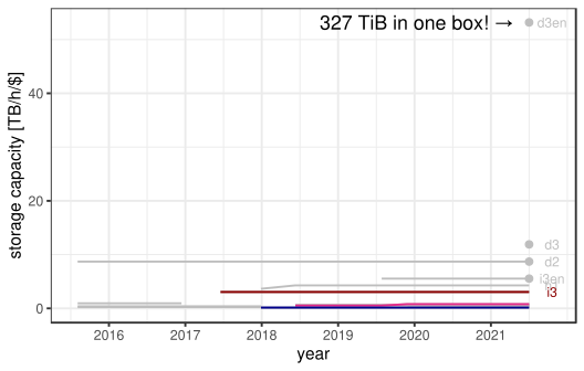
In terms of capacity per dollar, disk is still king and the d3en instance (introduced in December 2020) totally changed the game:

Network Bandwidth

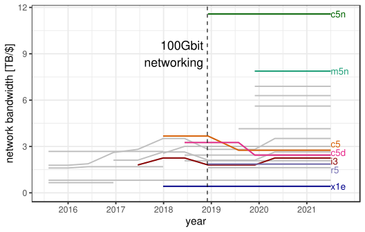
For network bandwidth, we see another major disruption, this time the introduction of 100GBit network instances:



The c5n instance, in particular, is clearly a game changer. It is only marginally more expensive than c5, but its network speed is 4 times faster.

Conclusions

These results show that the hardware landscape is very fluid and regularly we see major changes like the introduction of NVMe SSDs or 100 GBit networking. Truisms like "in distributed systems network bandwidth is the bottleneck" can become false! (Network latency is of course a different beast.) High-performance systems must therefore take hardware trends into account and adapt to the ever-evolving hardware landscape.

What Every Programmer Should Know About SSDs

Solid-State Drives (SSDs) based on flash have largely replaced magnetic disks as the standard storage medium. From the perspective of a programmer, SSDs and disks look very similar: both are persistent, enable page-based (e.g., 4KB) access through file systems and system calls, and have large capacities.

However, there are also important differences, which become important if one wants to achieve optimal SSD performance. As we will see, SSDs are more complicated and their performance behavior can appear quite mysterious if one simply thinks of them as fast disks. The goal of this post is to provide an understanding of why SSDs behave the way they do, which can help creating software that is capable of exploiting them. (Note that I discuss NAND flash, not Intel Optane memory, which has different characteristics.)

Drives not Disks

SSDs are often referred to as disks, but this is misleading as they store data on semiconductors instead of a mechanical disk. To read or write from a random block, a disk has to mechanically move its head to the right location, which takes on the order of 10ms. A random read from an SSD, in contrast, takes about 100us – 100 times faster. This low read latency is the reason why booting from an SSD is so much faster than booting from a disk.

Parallelism

Another important difference between disks and SSDs is that disks have one disk head and perform well only for sequential accesses. SSDs, in contrast, consist of dozens or even hundreds of flash chips ("parallel units"), which can be accessed concurrently.

SSDs transparently stripe larger files across the flash chips at page granularity, and a hardware prefetcher ensures that sequential scans exploit all available flash chips. However, at the flash level there is not much difference between sequential and random reads. Indeed, for most SSDs it is possible to achieve almost the full bandwidth with random page reads as well. To do this, one has to schedule hundreds of random IO requests concurrently in order to keep all flash chips busy. This can be done by starting lots of threads or using asynchronous IO interfaces such as libaio or io_uring.

Writing

Things get even more interesting with writes. For example, if one looks at write latency, one may measure results as low as 10us – 10 times faster than a read. However, latency only appears so low because SSDs are caching writes on volatile RAM. The actual write latency of NAND flash is about 1ms – 10 times slower than a read. On consumer SSDs, this can be measured by issuing a sync/flush command after the write to ensure that the data is persistent on flash. On most data center/server SSDs, write latency cannot be measured directly: the sync/flush will complete immediately because a battery guarantees persistence of the write cache even in the case of power loss.

To achieve high write bandwidth despite the relatively high write latency, writes use the same trick as reads: they access multiple flash chips concurrently. Because the write cache can asynchronously write pages, it is not even necessary to schedule that many writes simultaneously to get good write performance. However, the write latency cannot always be hidden completely: for example, because a write occupies a flash chip 10 times longer than a read, writes cause significant tail latencies for reads to the same flash chip.

Out-Of-Place Writes

Our understanding is missing one important fact: NAND flash pages cannot be overwritten. Page writes can only be performed sequentially within blocks that have been erased beforehand. These erase blocks have a size of multiple MB and therefore consist of hundreds of pages. On a new SSD, all blocks are erased, and one can directly start appending new data.

Updating pages, however, is not so easy. It would be too expensive to erase the entire block just to overwrite a single page in-place. Therefore, SSDs perform page updates by writing the new version of the page to a new location. This means that the logical and physical page addresses are decoupled. A mapping table, which is stored on the SSD, translates logical (software) addresses to physical (flash) locations. This component is also called Flash Translation Layer (FTL).

For example, let's assume we have a (toy) SSD with 3 erase blocks, each with 4 pages. A sequence of writes to pages P1, P2, P0, P3, P5, P1 may result in the following physical SSD state:

Block 0	P1 (old)	P2	P0	P3
Block 1	P5	P1	→
Block 2

Garbage Collection

Using the mapping table and out-of-place write, everything is good until the SSD runs out of free blocks. The old version of overwritten pages must eventually be reclaimed. If we continue our example from above by writing to pages P3, P4, P7, P1, P6, P2, we get the following situation:

Block 0	P1 (old)	P2 (old)	P0	P3 (old)
Block 1	P5	P1 (old)	P3	P4
Block 2	P7	P1	P6	P2

At this point we have no more free erase blocks (even though logically there should still be space). Before one can write another page, the SSD first has to erase a block. In the example, it might be best for the garbage collector to erase block 0, because only one of its pages is still in use. After erasing block 0, we make space for 3 writes and our SSD looks like this:

Block 0	P0	→
Block 1	P5	P1 (old)	P3	P4
Block 2	P7	P1	P6	P2

Write Amplification and Overprovisioning

To garbage collect block 0, we had to physically move page P0, even though logically nothing happened with that page. In other words, with flash SSDs the number of physical (flash) writes is generally higher than the number of logical (software) writes. The ratio between the two is called write amplification. In our example, to make space for 3 new pages in block 0, we had to move 1 page. Thus we have 4 physical writes for 3 logical writes, i.e., a write amplification of 1.33.

High write amplification decreases performance and reduces flash lifetime. How large write amplification is depends on the access pattern and how full the SSD is. Large sequential writes have low write amplification, while random writes are the worst case.

Let's assume our SSD is filled to 50% and we perform random writes. In steady state, wherever we erase a block, about half the pages of that block are still in use and have to be copied on average. Thus, write amplification for a fill factor of 50% is 2. In general, worst-case write amplification for a fill factor f is 1/(1-f):

f	0.1	0.2	0.3	0.4	0.5	0.6	0.7	0.8	0.9	0.95	0.99
WA	1.11	1.25	1.43	1.67	2.00	2.50	3.33	5	10	20	100

Because write amplification becomes unreasonably high for fill factors close to 1, most SSDs have hidden spare capacity. This overprovisioning is typically 10-20% of the total capacity. Of course, it is also easy to add more overprovisioning by creating an empty partition and never write to it.

Summary and Further Reading

SSDs have become quite cheap and they have very high performance. For example, a Samsung PM1733 server SSD costs about 200 EUR per TB and promises close to 7 GB/s read and 4 GB/s write bandwidth. Actually achieving such high performance requires knowing how SSDs work and this post described the most important behind-the-scenes mechanisms of flash SSDs.

I tried to keep this post short, which meant that I had to simplify things. To learn more, a good starting point is this tutorial, which also references some insightful papers. Finally, because SSDs have become so fast, the operating system I/O stack is often the performance bottleneck. Experimental results for Linux can be found in our CIDR 2020 paper.

Taming Deep Recursion

 When operating on hierarchical data structures, it is often convenient to formulate that using pairwise recursive functions. For example, our semantic analysis walks that parse tree recursively and transforms it into an expression tree. This corresponding code looks roughly like this:

 unique_ptr<Expression> analyzeExpression(AST* astNode) {  
   switch (astNode->getType()) {  
    case AST::BinaryExpression: return analyzeBinaryExpression(astNode->as<BinaryExpAST>());  
    case AST::CaseExpression: return analyzeCaseExpression(astNode->as<CaseExpAST>());  
    ...  
   }  
 }  
 unique_ptr<Expression> analyzeBinaryExpression(BinaryExpAST* astNode) {  
   auto left = analyzeExpression(astNode->left);  
   auto right = analyzeExpression(astNode->right);  
   auto type = inferBinaryType(astNode->getOp(), left, right);  
   return make_unique<BinaryExpression>(astNode->getOp(), move(left), move(right), type);  
 }  

It recursively walks the tree, collects input expressions, infers types, and constructs new expressions. This works beautifully until you encounter a (generated) query with 300,000 expressions, which we did. At that point our program crashed due to stack overflow. Oops.

Our first mitigation was using __builtin_frame_address(0) at the beginning of analyzeExpression to detect excessive stack usage, and to throw an exception if that happens. This prevented the crash, but is not very satisfying. First, it means we refuse a perfectly valid SQL query "just" because it uses 300,000 terms in one expression. And second, we cannot be sure that this is enough. There are several places in the code that recursively walk the algebra tree, and it is hard to predict their stack usage. Even worse, the depth of the tree can change due to optimizations. For example, when a query has 100,000 entries in the from clause, the initial tree is extremely wide but flat. Later, after we have stopped checking for stack overflows, the optimizer might transform that into a tree with 100,000 levels, again leading to stack overflow. Basically, all recursive operations on the algebra tree are dangerous.

Now common wisdom is to avoid recursion if we cannot bound the maximum depth, and use iteration with an explicit stack instead. We spend quite some time thinking about that approach, but the main problem with that is that it makes the code extremely ugly. The code snippet above is greatly simplified, but even there an explicit stack would be unwieldy and ugly if we have to cover both binaryExpression and caseExpression using one stack. And the code gets cut into tiny pieces due to the control flow inversion required for manual stacks. And all that to defend against something that nearly never happens. We were unhappy with that solution, we wanted something that is minimal invasive and created overhead only in the unlikely case that a user gives us an extremely deep input.

One mechanism that promises to solve this problem is -fsplit-stack. There, the compiler checks for stack overflows in the function prolog and creates a new stack segment if needed. Great, exactly what we wanted! We can handle deep trees, no code change, and we only create a new stack if we indeed encounter deep recursion. Except that it is not really usable in practice. First, -fsplit-stack is quite slow. We measured 20% overhead in our optimizer when enabling split stacks, and that in cases where we did not create any new stacks at all. When -fsplit-stack does create new stacks it is even worse. This is most likely a deficit of the implementation, one could implement -fsplit-stack much more efficiently, but the current implementation is not encouraging. Even worse, clang produces an internal compiler error when compiling some functions with -fsplit-stack. Nobody seems to use this mechanism in production, and after disappointing results we stopped considering -fsplit-stack.

But the idea of split stacks is clearly good. When encountering deep recursion we will have to switch stacks at some point. After contemplating this problem for some time we realized that boost.context offers the perfect mechanism for switching stacks: It can start a fiber with a given stack, and switching between fibers costs just 19 cycles. By caching additional stacks and their fibers in thread-local data structures we can provide our own implementation of split stacks that is fast and supports arbitrary code. Without compiler support the split stack mechanism is visible, of course, but that is fine in our code. We have only a few entry points like analyzeExpression that will be called over and over again during recursion, and checking there is enough. Code wise the mechanism is not too ugly, it needs two lines of code per recursion head and looks like

 unique_ptr<Expression> analyzeExpression(AST* astNode) {  
   if (StackGuard::needsNewStack())  
    return StackGuard::newStack([=]() { return analyzeExpression(astNode); });  
   ... // unchanged  
 }  

Note that the lambda argument for newStack will be called from within the new stack, avoiding the stack overflow. When the lambda returns the mechanism will use boost.context to switch back to the previous stack. The performance impact of that mechanism is negligible, as 1) we do not check for overflows all the time but only in the few places that we know are central to the recursive invocations, like analyzeExpression here, 2) stack overflows are extremely rare in practice, and we only pay with one if per invocation is no overflow happens, and 3) even if they do happen, the mechanism is reasonably cheap. We cache the child stacks, and switching to a cached stack costs something like 30 cycles. And we never recurse in a hot loop.

It took us a while to get there, but now we can handle really large queries without crashing. Just for fun we tried running a query with 100,000 relations in the from clause. Fortunately our optimizer could already handle that, and now the rest of the system can handle it, too. And that with nice, intuitive, recursive code, at the small price of two lines of code per recursion head.

C++ Concurrency Model on x86 for Dummies

Since C++11, multi-threaded C++ code has been governed by a rigorous memory model. The model allows implementing concurrent code such as low-level synchronization primitives or lock-free data structures in a portable fashion. To use the memory model, programmers need to do two things: First, they have to use the std::atomic type for concurrently-accessed memory locations. Second, each atomic operation requires a memory order argument with six options determining the concurrency semantics in terms of which re-orderings are allowed. (Some operations even allow specifying two memory orders!)

While there are a number of attempts to describe the model, I always found the full semantics very hard to understand and consequently concurrent code hard to write and reason about. And since we are talking about low-level concurrent code here, making a mistake (like picking the wrong memory order) can lead to disastrous consequences.

Luckily, at least on x86, a small subset of the full C++11 memory model is sufficient. In this post, I'll present such a subset that is sufficient to write high-performance concurrent code on x86. This simplification has the advantage that the resulting code is much more likely to be correct, without leaving any performance on the table. (On non-x86 platforms like ARM, code written based on this simplified model will still be correct, but might potentially be slightly slower than necessary.) 

There are only six things one needs to know to write high-performance concurrent code on x86.

1. Data races are undefined

If a data race occurs in C++, the behavior of the program is undefined. Let's unpack that statement. A data race can be defined as two or more threads accessing the same memory location with at least one of the accesses being a write. By default (i.e., without using std::atomic), the compiler may assume that no other thread is concurrently modifying memory. This allows the compiler to optimize the code, for example by reordering or optimizing away memory accesses. Consider the following example:

void wait(bool* flag) {
    while (*flag);
}

Because data races are undefined, the compiler may assume that the value behind the pointer flag is not concurrently modified by another thread. Using this assumption, gcc translates the code to a return statement while clang translates it to an infinite loop if flag is initially true. Both translations are likely not what the code intends. To avoid undefined code, it is necessary use std::atomic for variables where race conditions may happen:

void wait(std::atomic<bool>* flag) {
    while (*flag); // same as while(flag->load(std::memory_order_seq_cst));
}

*flag is equivalent to flag.load(std::memory_order_seq_cst), i.e., the default memory order is sequential consistency. Sequential consistency is the strongest memory order guaranteeing that atomic operations are executed in program order. The compiler is not allowed to reorder memory operations or optimize them away.

2. Sequentially-consistent loads are fast

Making the flag atomic may seem expensive, but luckily atomic loads are cheap on x86. Indeed, our wait function is translated to a simple loop with a simple MOV instruction, without any barrier/fence instruction. This is great as it means that on x86 an atomic, sequentially-consistent load can be just as fast as a normal load. It also means that on x86 there is no performance benefit of using any weaker memory order for atomic loads. For loads all memory orders are simply translated to MOV.

3. Sequentially-consistent stores are slow

While sequentially-consistent atomic loads are as cheap as normal loads, this is not the case for stores, as can be observed from the following example:

void unwait(std::atomic<bool>* flag) {
    *flag = false; // same as flag->store(false, std::memory_order_seq_cst);
}

As with atomic loads, atomic stores are sequentially consistent if no explicit memory order is specified. In clang and gcc 10, the store translates to an XCHG instruction rather than a MOV instruction (older gcc versions translate it to a MOV plus MFENCE.). XCHG and MFENCE are fairly expensive instructions but are required for sequentially consistent stores on x86. (The CPU's store buffer must be flushed to L1 cache to make the write visible to other threads through cache coherency.)

4. Stores that can be delayed can benefit from the release memory order

Because sequentially-consistent stores are fairly expensive, there are situations where a weaker memory order can improve performance. A common case is when the effect of a store can be delayed. The classical example is unlocking a mutex. The unlocking thread does not have to synchronously wait for the unlocking to become visible, but can continue executing other instructions. Another way of saying this is that it is correct to move instructions into the critical section, but not out of it. In C++, this weaker form of store consistency is available through the release memory order.

In our unwait example, the store can indeed be delayed, which is why we can use the release memory order for the store:

void unwait(std::atomic<bool>* flag) {
    flag->store(false, std::memory_order_release);
}

This code is translated to a simple MOV instruction, which means it can be as efficient as a non-atomic store.

5. Some atomic operations are always sequentially consistent

Besides loads and stores, std::atomic also offers the high-level atomic operations compare_exchange, exchange, add, sub, and, or, xor. On x86, these are always directly translated to sequentially-consistent CPU instructions. This means that there is no performance benefit from specifying weaker memory orders on any of these operations. (An atomic increment with release semantics would be useful in many situations, but alas is not available.)

6. Scalable code should avoid cache invalidations

I mentioned above that sequentially-consistent loads and release stores may be as cheap as non-atomic loads/store. Unfortunately, this is not always the case. Because CPUs have per-core caches, the performance of concurrent programs depends on the dynamic access pattern. Every store has to invalidate any cached copies of that cache line on other cores. This can cause parallel implementations to be slower than single-threaded code. Therefore, to write scalable code, it is important to minimize the number of writes to shared memory locations. A positive way of saying this is that as long as the program does not frequently write to memory locations that are frequently being read or written, the program will scale very well. (Optimistic lock coupling, for example, is a general-purpose concurrency scheme for synchronizing data structures that exploits this observation.)

Summary

The full C++ memory model is notoriously hard to understand. x86, on the other hand, has a fairly strong memory model (x86-TSO) that is quite intuitive: basically everything is in-order, except for writes, which are delayed by the write buffer. Exploiting x86's memory model, I presented a simplified subset of the C++ memory model that is sufficient to write scalable, high-performance concurrent programs on x86.